Tracking our Experiments
"Remember kids, the only difference between screwing around and science is writing it down!" — Adam Savage
Before now we've kind of gotten away with not keeping track in too much detail because it's largely been tests and individual experiments. But, that's going to change now. As we start to iterate over different features it becomes more important than ever that we do two things:
- Change only one thing at a time
- Log results of how things changed
Why is this so important? Well, if we change more than one thing at a time how do we know what improved the results? Maybe one thing made it worse and another made it better? It's critical that we take an experimental approach here so that we can see what improves things to drive further experimentation and refinement. Also, for posterity it's critical we write things down - Everyone has been in the situation on Friday afternoon where they're sure they'll remember something on Monday. They don't. We don't want to be in that situation so... MLFlow
Where does MLFlow live?
We actually have two different choices here with different trade-offs for how we want to setup MLFlow:
| Approach | Pros | Cons |
| Run on a Server | + Always available, allows multiple collaborators, more "production-like" | - Cost of running a server, maintenance overhead |
| Run Locally | + Super quick setup, zero cost | - Multiple collaborators is *difficult* |
For our purposes right now, as a solo-developer on this project it makes a lot more sense to set up locally for now because it means we don't have the overhead of managing a separate server and DB instance. When we get to the point of having multiple collaborators later on we can copy all the runs and artifacts with the following script:
python -m mlflow.store.artifact.cli copy-artifacts \
    --src-uri file:./mlruns \
    --dst-uri s3://your-bucket/mlruns
And there is a community written package that also handles bulk experiment migration as well cleanly at mlflow-export-import. So, in summary we've made our decision for where to host, all we need to do now is get it setup.
What we do is setup a python virtual environment, install it with pip install mlflow and then run it with the following:
mlflow server \
  --backend-store-uri sqlite:///mlruns.db \
  --default-artifact-root ./mlartifacts \
  --host 127.0.0.1 \
  --port 5000
Setting Up Folds
So far we've been evaluating against a single validation set, but we can do better. Cross-validation gives us a more robust picture of model performance by evaluating across multiple slices of the data, but not all cross-validation strategies are created equal for time-series problems.
Random K-Fold is out immediately. Randomly splitting F1 race data across folds leaks future races into training, which fundamentally invalidates the evaluation.
Expanding window (sklearn's TimeSeriesSplit) is better as it respects temporal ordering, but the training set grows with each fold. That means later folds have seen significantly more data than earlier ones, so differences in fold performance are harder to attribute purely to the validation window.
Rolling window is what we're going to use. We define a fixed training window of 10 seasons and slide it forward one year at a time, always validating on the season immediately after the window. Every fold trains on the same volume of data, and old seasons age out as the window moves forward. That last point is particularly relevant for F1: the sport has changed so dramatically across regulation eras that 1990s race data is of questionable value when predicting results today, so we're not too worried about losing it.
years = sorted(training_base_race_data_df["year"].unique())

train_window = 10
val_window = 1

folds = []
for i in range(len(years) - train_window - val_window + 1):
    train_years = years[i : i + train_window]
    val_years   = years[i + train_window : i + train_window + val_window]
    folds.append((train_years, val_years))
With our data running from 1991 to 2024, this produces 24 folds, each training on a decade of seasons and validating on the next. The mean AUC and Brier score across all folds become our headline numbers for comparing runs in MLFlow going forward.
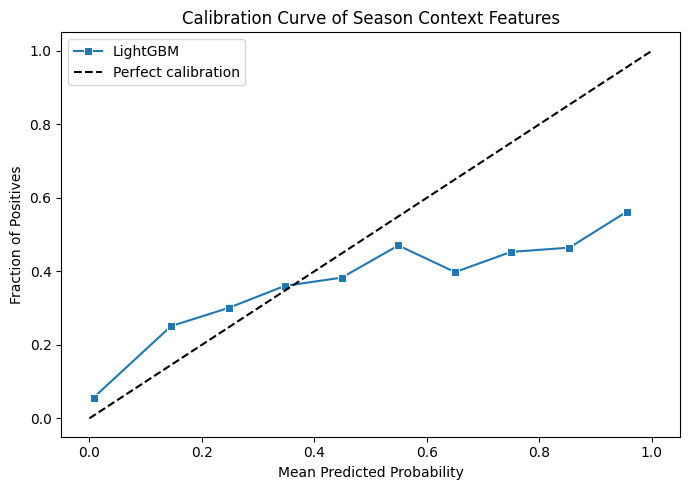
The key numbers for us going on now should be the mean AUC and mean brier score, which will hopefully be more stable due to the averaging.
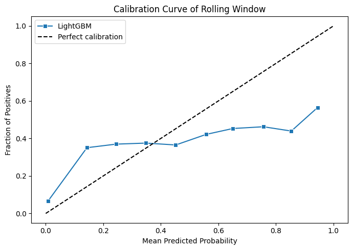
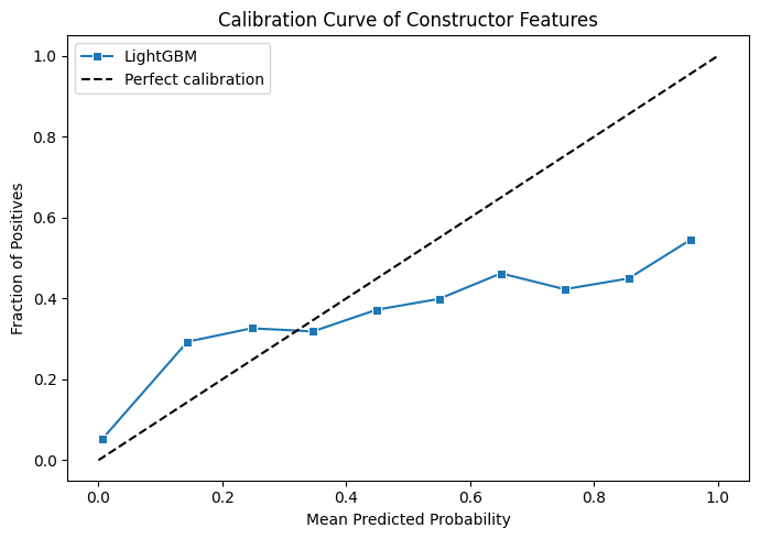
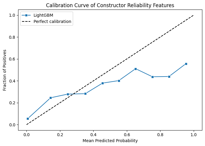
This is good news! We can see that from the averaging of the now 24 different validation sets that we have the calibration curve is looking a lot smoother. This means that we should be subject to less volatility during testing. But, we have another big problem we've left unaddressed.
Class Imbalances
In Part 2, we talked briefly about how the model was able to dump almost everything into "No podium" and still be somewhat accurate. This was mostly down to the fact that our dataset, by design almost, heavily suffers from class imbalance.
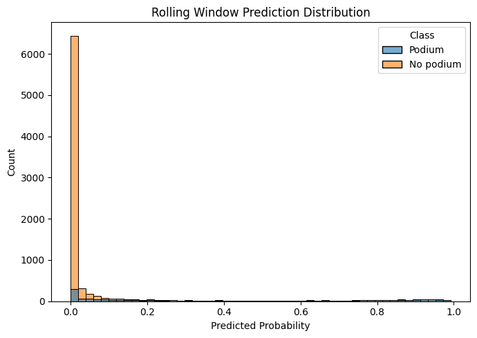
Fortunately, LightGBM has a knob that we can turn to hopefully mitigate most of that problem. That knob in our case is scale_pos_weight.
We have a dataset that (at least in 2025) consists of 20 drivers and 3 podiums per race, meaning that we have 17 non-podium results for every 3 podium finishes. The recommended value for scale_pos_weight is the ratio of negative to positive samples, so we set it to 17/3 ≈ 5.67.
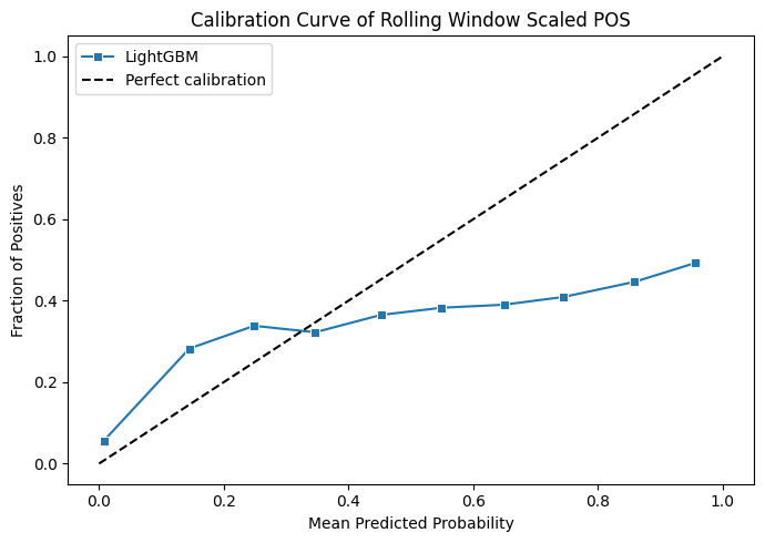
How does it work? LightGBM multiplies the weight of each positive sample (a podium finish) by that factor, so the minority class punches at roughly the same weighted value as the majority class during training.
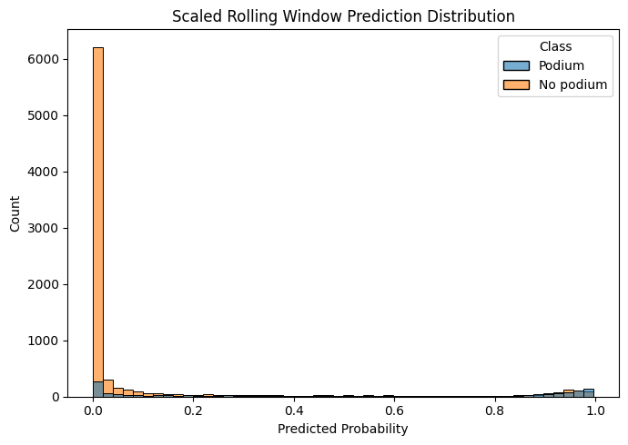
The good news is that this seems to have fixed our class imbalance problem to some degree, yes the model does still strongly favour "no podium" a lot of the time but we have some degree of more even distribution now. It's also had the added benefit of smoothing out the probability curve a bit more as well.
Making Features
Okay! Now with all of that out of the way, we've got our rolling window validation so our validation should be more stable now, and also we've resolved our imbalance problem as best as we can. So now we need to decide what features should we make that capture if someone's going to podium?
Rolling Driver Podium Rates
It's probably a good bet that a driver who has been on the podium recently is going to be on the podium again. We can probably break this into three different timespans
- Short term - The last 3 races
- Medium term - The last 5 races
- Long term (at least for F1 drivers...) - The last 10 races
Each of those gives us a different picture about how the driver will perform in future, after all someone who does well on the last 10 but badly on the last 3 might be having a bumpy patch. Or someone who is doing poorly in the last 10 but great on the last 5 might have had a big upgrade. Either way, they all tell us something interesting
So, what we do is we:
- Sort the drivers by driver id, year and round (important for later because we're using .rolling()
- Group the drivers by driver ID, and take the "podiumFinish" feature
- Shift back 1 to avoid the current race, and then take a rolling average of the last 3 races
- Repeat this for 3, 5 and 10 races
training_base_driver_en_1_data_df = (
    training_base_race_data_df
    .sort_values(["driverId", "year", "round"])
    .copy()
)

training_base_driver_en_1_data_df["driver_podium_rate_3"] = (
    training_base_driver_en_1_data_df.groupby("driverId", observed=True)["podiumFinish"]
    .transform(lambda x: x.shift(1).rolling(3, min_periods=1).mean())
)

training_base_driver_en_1_data_df["driver_podium_rate_3"] = training_base_driver_en_1_data_df["driver_podium_rate_3"].fillna(0)
training_base_driver_en_1_data_df.head()
Great, now what we do with these new features is to put them back into training and see how our model performs.
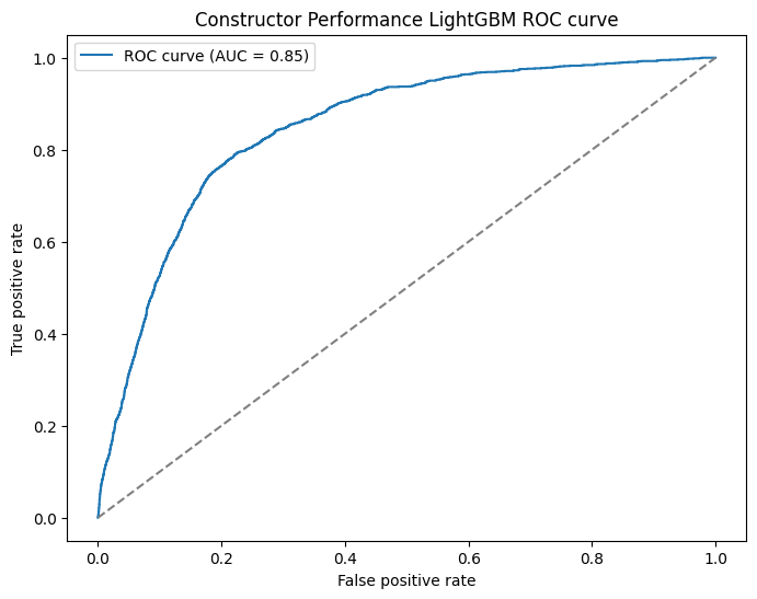
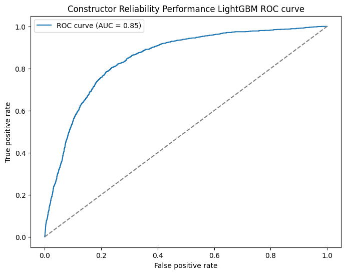
| AUC/ROC | Brier Score |
| 0.8440 (baseline: 0.79) | 0.1174 (baseline: 0.12) |
| +0.0324 from previous | -0.0041 from previous |
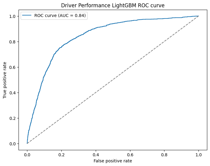
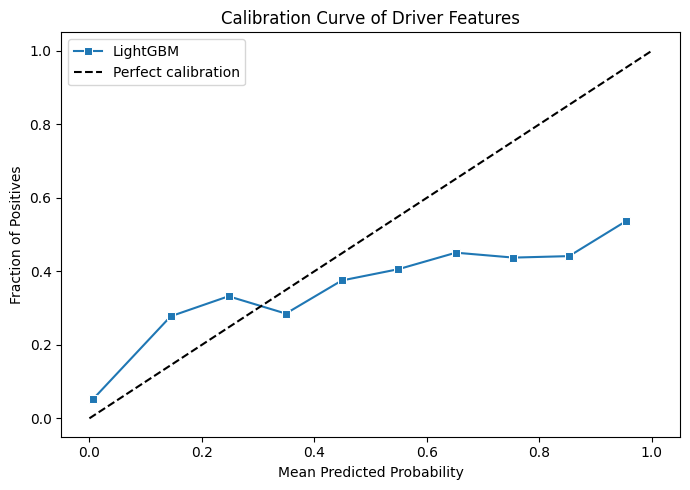
These graphs are looking a lot healthier! Our ROC curve looks a lot more consistent now and the calibration curve of probability is also looking more consistently close to the line as well. We can surmise that in terms of both the probabilities of the drivers to podium and which drivers podium are both slightly more accurate with the new features.
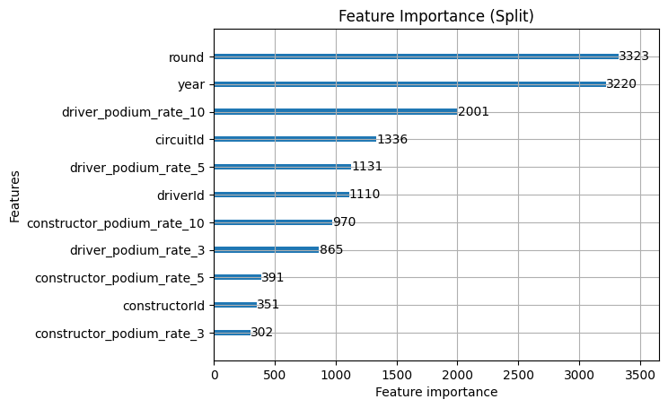
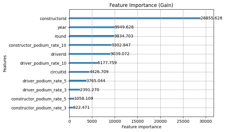
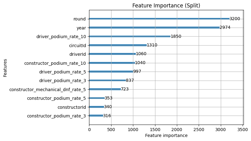
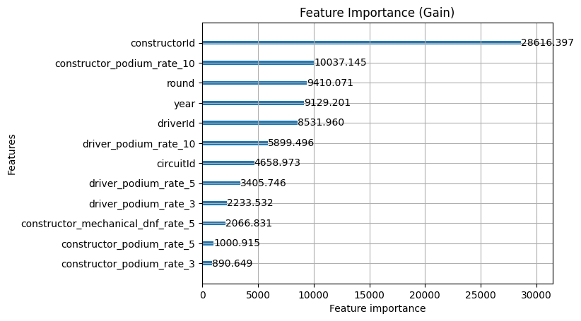
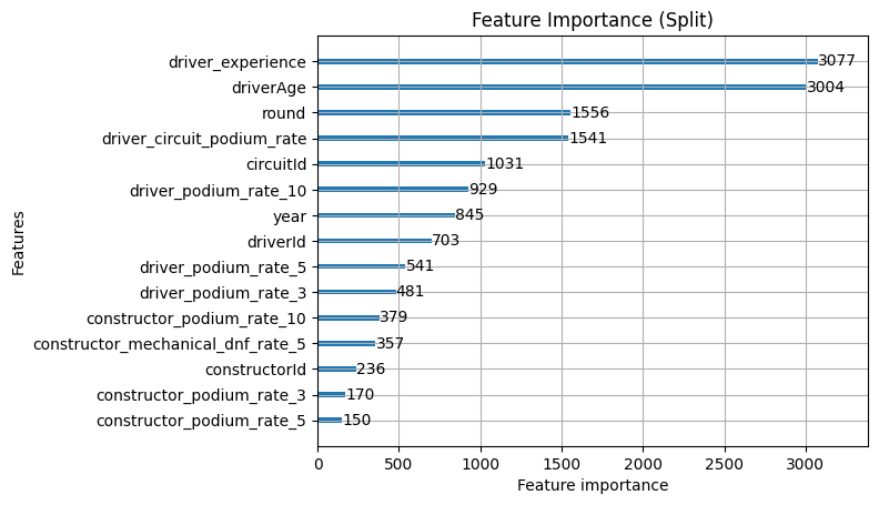
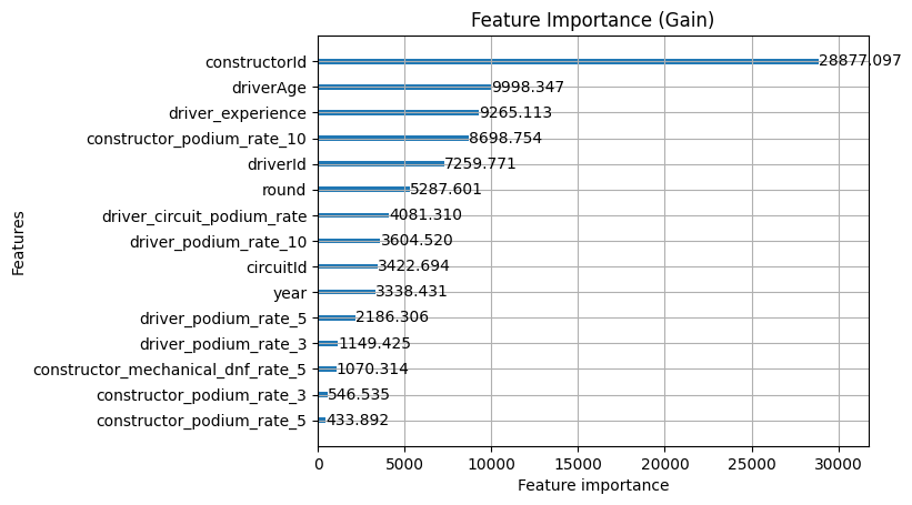
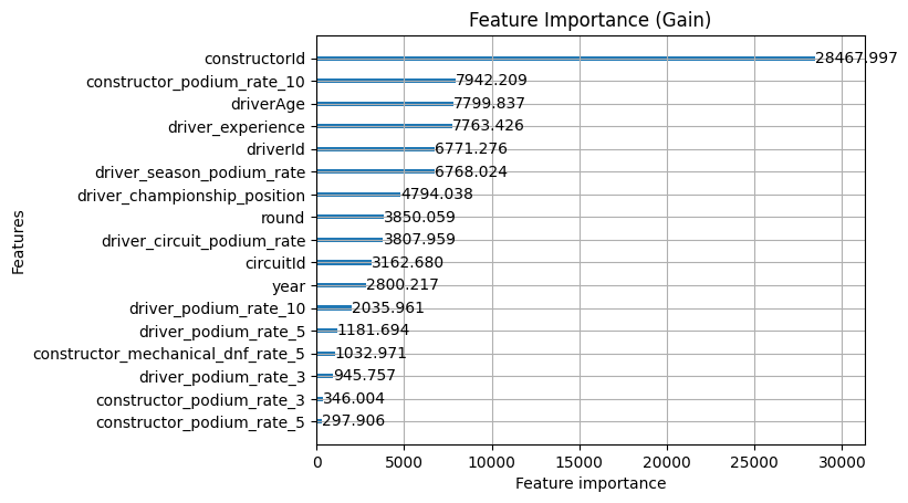
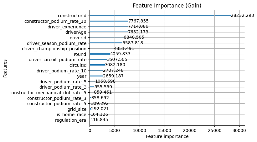
We've also got another tool to understand these numbers it's called feature importance graphs. They come in two forms that we're interested in right now, splits which tell us how many times a feature was used to split a tree and gain which tells us the average improvement of the loss function based on that feature. Split can get artificially inflated especially if it's a low level tie-breaker and gain also gets inflated if you have high-cardinality features like constructor id, because those big top level splits theoretically are very good. Looking at both of them together though gives us a great picture of what's going on.
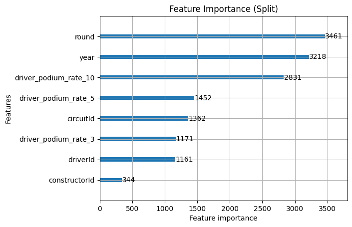
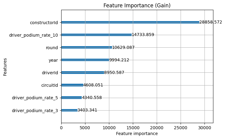
So, there are a couple of things to unpack here from these graphs:
- Constructor ID gets a huge gain but tiny split, so it's likely used as a top level feature and has that inflation problem, there is information here but we're likely not tapping into it enough yet
- Round & year are used for a lot of splits, but the value is middling so it's likely being used as a tie breaker rather than providing a lot of value on their own just yet
- The driver podium rate for the last 10 races is very high in both so it's providing great value
But overall it's a success so far! Let's keep going.
Rolling Constructor Podium Rates
Previously, we looked at the drivers. But we could also look at the constructors too! After all which constructors win is the average of the drivers skill yes, but also the car, the engineering, the research.
So, we take a look at the constructor podium rates for the same 3, 5 and 10 race cycles to see if there are patterns. There's an important note we're building on top of the previous features here. The reason for this is that yes, we could isolate them to try and see the effects of those features on their own, but what we'd actually be doing is forcing the model to compensate for the lack of the driver features by pushing them into these constructor features or other features, that makes our process less, not more clear.
training_base_driver_en_2_data_df["constructor_podium_rate_3"] = (
    training_base_driver_en_2_data_df.groupby("constructorId", observed=True)["podiumFinish"]
    .transform(lambda x: x.shift(1).rolling(3, min_periods=1).mean())
)

training_base_driver_en_2_data_df["constructor_podium_rate_3"] = training_base_driver_en_2_data_df["constructor_podium_rate_3"].fillna(0)
training_base_driver_en_2_data_df.head()
So, how do we do with this feature added?
| AUC/ROC | Brier Score |
| 0.8463 (baseline: 0.79) | 0.1167 (baseline: 0.12) |
| +0.0023 from previous | -0.0007 from previous |
A small amount better, not worse but still. Probably not the improvement that we were hoping for honestly. Looking at the feature importance will tell us the whole story.
Even though the performance itself didn't see a big hike, we do actually see patterns here which are significantly healthier in the model, and likely more robust as well such as:
- driver_podium_rate_10 has been diluted a bit when the constructor features were added. The constructor podium rates are absorbing variance it was previously carrying alone, which makes sense given how correlated driver and constructor form are.
- constructor_podium_rate_10 immediately earns its place. Fourth on gain the 10 race window is still the strongest, but this makes sense for constructors as well because the cars change on longer cycles
- constructorId gain doesn't change. The rolling constructor rates are capturing something genuinely different from the raw identity signal.
- The split counts are more evenly distributed meaning that the constructor features have taken splits from the driver features without any single feature dominating, suggesting the model is using the full feature set in a balanced way.
In summary, even though we didn't get a bunch more performance from our model, it is more healthy and hopefully more stable.
Reliability
As we discussed in the EDA, we treat a DNF as a failure to get a podium. Therefore, DNF's for things that we can predict such as mechanical reliability, we can't predict an accident however, and nobody predicts Logan Sargent so, we'll exclude that from this feature. What we want to build here is a rolling 5 race car reliability metric similar to race and constructor.
What this should tell is "Is a drivers ability to get a podium affected by the reliability of the car?" We'll also keep out things like being lapped and fires because they're ambiguous so they're best left out.
non_mechanical_statuses = [
    # Finished / classified
    "Finished",
    "+1 Lap", "+2 Laps", "+3 Laps", "+4 Laps", "+5 Laps",
    "+6 Laps", "+7 Laps", "+8 Laps", "+9 Laps", "+10 Laps",
    "+11 Laps", "+12 Laps", "+13 Laps", "+14 Laps", "+15 Laps",
    "+16 Laps", "+17 Laps", "+18 Laps", "+19 Laps", "+20 Laps",
    "+21 Laps", "+22 Laps", "+23 Laps", "+24 Laps", "+25 Laps",
    "+26 Laps", "+29 Laps", "+30 Laps", "+38 Laps", "+42 Laps",
    "+44 Laps", "+46 Laps", "+49 Laps",

    # Racing incidents
    "Accident", "Collision", "Collision damage", "Spun off", "Fatal accident",

    # Driver / personal
    "Physical", "Injured", "Injury", "Driver unwell", "Eye injury",
    "Illness", "Safety belt", "Driver Seat", "Seat",

    # Regulatory / administrative
    "Disqualified", "Excluded", "Underweight", "107% Rule",
    "Did not qualify", "Did not prequalify", "Not classified",
    "Withdrew", "Not restarted",

    # Ambiguous — excluded to keep data clean
    "Retired", "Damage", "Debris", "Fire", "Safety", "Safety concerns",

    # Pit / logistics
    "Fuel Rig",
]

mechanical_dnf_ids = status_df[
    ~status_df["status"].isin(non_mechanical_statuses)
]["statusId"]
With this feature added, and retraining the model with all of the previous features included we get
| AUC/ROC | Brier Score |
| 0.8480 (baseline: 0.79) | 0.1145 (baseline: 0.12) |
| +0.004 from previous | -0.0029 from previous |
Again, very minor improvements on the ranking and probability accuracy of the model. We largely see incremental improvements nothing amazing but, it's moving in the right direction. Then we go to the feature importance to see the rest of the picture to explain.
- Constructor ID hasn't moved: This is good in that it means we're adding new features rather than redundant ones
- Constructor_podium_rate_10 gets a small boost: This is likely down to the reliability of constructors absorbing some of what constructor id was doing before to identify unreliable constructors. This means the podium rate can do its job better because it only has to track this now
Ultimately, including mechanical DNF for constructors was additive, but not really transformative. We'd honestly benefit from exploring this a bit more because if this new feature correlates strongly with constructor ID then we know that the constructor ID is already doing this job for us
Driver Profile
We know that drivers have an impact, we got this from the podium rates of the drivers but we can probably dig a little deeper into drivers feature wise to expose the detail to the model. We know for example that drivers performance typically follows an inverted U shape (Unless you're Lewis Hamilton). This is probably a mixture of both a drivers age, and their experience.
We can capture their age really easily by just taking the difference between the race date and their date of birth, general experience we'll track as the rolling number of races that they have performed in over their career to date. Another thing to consider is per track experience. Some drivers are just more familiar with certain tracks and surely that plays into some degree of performance (Charles I'm sure is familiar with Monaco...). So, we'll set up these features as:
- driverAge: The age in years of the driver at the time of the race
- driver_experience: The cumulative count of the drivers total races
- driver_circuit_podium_rate: The podium rate for the driver on the specific track
driver_experience is a simple cumulative count of races started, we use cumcount() rather than a rolling window because we want the total career count, not a recent snapshot.
For driver_circuit_podium_rate there's an important note. We need to use an expanding mean rather than a fixed rolling window. Some driver-circuit combinations only appear a handful of times across an entire career, so a fixed window like rolling(3) would produce NaN for the first two visits and only give a meaningful value from the third appearance onwards. expanding() instead takes the mean of all prior visits however few there are, so you always get a valid number.
training_base_driver_en_4_data_df["driver_circuit_podium_rate"] =
  (training_base_driver_en_4_data_df.groupby(["driverId", "circuitId"], observed=True)["podiumFinish"]
    .transform(lambda x: x.shift(1).expanding().mean()))
| AUC/ROC | Brier Score |
| 0.8359 (baseline: 0.79) | 0.1141 (baseline: 0.12) |
| -0.0121 from previous | -0.0004 from previous |
Our AUC dropped marginally, meaning that we're slightly less able to tell who will podium vs who will not. Our brier score dropped as well but the change is likely just noise because it's so tiny. Age and experience are quite coarse features, someone with 50 races might be a seasoned veteran or... Lance Stroll. Circuit specific experience is interesting but it might already be being captured by driverId and circuitId. We'll explore the feature importance to see.
Interestingly, we do see that the new features are being used. They're quite high up in split and gain, but we need to consider this in the context that the AUC and Brier didn't really improve. Likely what we're seeing happen is that it's using them because they're available but they're not really adding anything new, just presenting what the model already knew about driverId and year in a different way
Season Context
The rolling podium rates we have give us a sense of recent driver form, but they don't account for the context of the season they're currently in. A driver on a hot streak in a dominant car mid-season is a very different proposition to a driver who happened to podium a few times two years ago. driver_season_podium_rate captures this by tracking the driver's podium rate within the current season up to but not including the current race, giving the model a view of whether a particular driver and car package has genuinely found its feet that season.
Championship position is arguably the most information-dense single feature we can give the model. By the time you reach any given race, the standings encode a huge amount about that driver: how quick their car is, how reliably it finishes, and how consistently the driver themselves has been performing. It's a composite signal that would otherwise take several features to approximate. A driver sitting third in the championship before a race weekend is telling the model something meaningful that neither constructorId nor the rolling rates fully capture on their own.
We derive it by taking the cumulative points per driver within each season up to the previous race using shift(1).cumsum(), then ranking within each race weekend. There's an important detail in how we handle the first race of the season where no prior points exist, we can't fill with zero because that would imply the driver is leading the championship rather than being unranked, which would actively mislead the model. Instead we fill with the length of the grid, placing unranked drivers at the back where they belong.
training_base_driver_en_5_data_df["driver_championship_position"] = (
  training_base_driver_en_5_data_df.groupby("raceId")["driver_championship_position"]
    .transform(lambda x: x.fillna(len(x)))
)| AUC/ROC | Brier Score |
| 0.8450 (baseline: 0.79) | 0.1132 (baseline: 0.12) |
| +0.0091 from previous | -0.0009 from previous |

The AUC nudging up by 0.0091 tells us these features are adding genuine ranking signal rather than just restating what the model already knew. Brier is noise as usual, but at least we're not breaking calibration as we go. We're now sitting at 0.8450 against a baseline of 0.79, which is a solid cumulative gain.
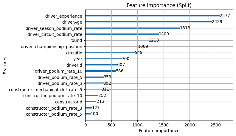
Both new features landed solidly. driver_season_podium_rate in particular came in with high gain and split, higher gain than driverId itself. This suggests it's carrying genuinely new signal about current-season form that nothing else was capturing.
driver_championship_position is more modest but still has a meaningful presence, comparable to where driver_circuit_podium_rate sat in the previous iteration.
The more telling story is what happened to the existing features. round, year and driver_podium_rate_10 all dropped noticeably, and that's actually a good sign. The new features appear to be absorbing load those were previously carrying as proxies for season context. The model is now getting that signal from features that actually represent it directly rather than approximating it through race number and calendar year.
In summary, it's not a paradigm change sure, but the model keeps getting healthier.
Race & Circuit Context
So far our features have all been about performance history. These next four are a bit different. They're about the structural conditions of the race itself, things that affect every driver on the grid regardless of form.
The most significant of these is regulation_era. We've talked before about year being a blunt instrument, the model has been forced to rediscover regulation boundaries on its own through raw calendar year. Encoding era directly as a categorical gives it that context explicitly. A hybrid-era Mercedes and a ground-effect-era Ferrari are fundamentally different machines.
circuit_type follows similar logic. Street circuits like Monaco or Baku produce structurally different racing which means the podium distribution looks meaningfully different to a permanent circuit. Flagging this explicitly lets the model treat them differently without having to learn it purely from circuitId.
grid_size addresses something more mechanical. The base rate of a podium finish is simply different in a field of 16 cars versus 26. Without this the model has no way to account for how the raw probability of a top-three finish shifts across eras.
is_home_race is the most speculative of the four. The effect is likely small, but home races carry real motivational weight for drivers and occasionally extra resource commitment from teams.
In order to do the tagging for regulation era and circuit type as well as matching the country to nationality we just use python maps for this.
| AUC/ROC | Brier Score |
| 0.8441 (baseline: 0.79) | 0.1127 (baseline: 0.12) |
| -0.0009 from previous | -0.0005 from previous |
Both movements are well within noise territory. regulation_era and is_home_race genuinely don't add anything, and we'll see that reflected in the importance charts shortly.
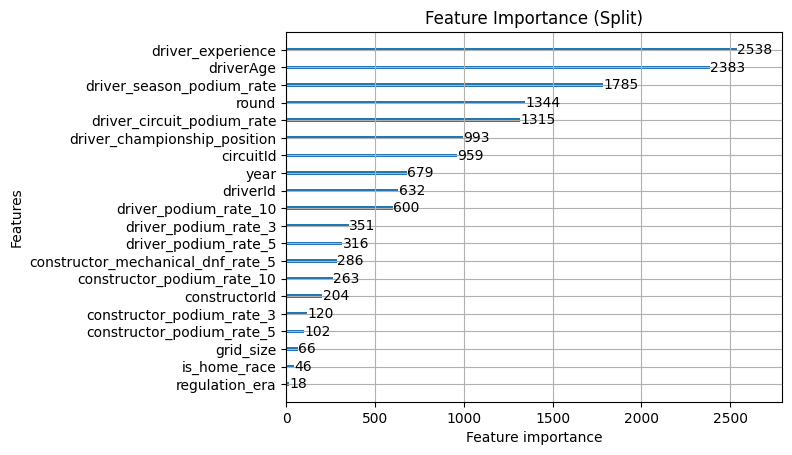
The importance charts confirm it. regulation_era and is_home_race sit at the very bottom of both gain and split, and grid_size is barely above them. The existing features are otherwise stable compared to the previous iteration, which tells us the race context additions didn't displace anything useful.
We've probably got all we can now out of feature engineering, so we'll move on.
Optimizing Hyperparameters
When we started, there wasn't a real benefit to trying out different hyperparameters because we'd likely end up overtuning and therefore overfitting on a single combination. Plus there is the overhead of having to tune for every single experiment. But now that we're in a more stable place with a good amount of features it's time to explore that.
We're going to use Optuna. What is it? Why are we using it? Firstly we need to talk about optimization methods.
The most basic approach would be Grid Search, in this case what we would do is define different values for each of the different parameters. This works okay for small amounts of tuning but we run in a different problem fast. It's called the curse of dimensionality. If we have 3 parameters and 3 different values we have 3^3 = 27 different models to tune. If we want to add an extra 2 values and 2 parameters? This is now 5^5 = 3,125. That's a 115x increase in the number of models to tune.
A better approach is Bayesian Search. I'm oversimplifying a lot, but effectively what we do is define the same grid but instead of brute forcing the problem, we set up a theoretical model. We see how our parameters perform against a loss function we've defined to see "how well" we do. We then use that information to decide what parameters to change. When you see the word "Bayesian" just think "Updating the problem with new information".
def objective(trial):
    params = {
        "objective": "binary",
        "verbose": -1,
        "n_estimators": trial.suggest_int("n_estimators", 100, 1000),
        "learning_rate": trial.suggest_float("learning_rate", 0.01, 0.3, log=True),
        "num_leaves": trial.suggest_int("num_leaves", 20, 150),
        "min_child_samples": trial.suggest_int("min_child_samples", 10, 100),
        "scale_pos_weight": trial.suggest_float("scale_pos_weight", 1.0, 10.0),
        "subsample": trial.suggest_float("subsample", 0.5, 1.0),
        "colsample_bytree": trial.suggest_float("colsample_bytree", 0.5, 1.0),
    }

    fold_briers = []

    for fold, (train_years, val_years) in enumerate(folds):
        train_mask = final_f1_feature_df["year"].isin(train_years)
        val_mask   = final_f1_feature_df["year"].isin(val_years)

        X_train_fold, y_train_fold = X[train_mask], y[train_mask]
        X_val_fold,   y_val_fold   = X[val_mask],   y[val_mask]

        model = lgb.LGBMClassifier(**params)
        model.fit(X_train_fold, y_train_fold)
        preds = model.predict_proba(X_val_fold)[:, 1]
        fold_briers.append(brier_score_loss(y_val_fold, preds))

    return sum(fold_briers) / len(fold_briers)

study = optuna.create_study(direction="minimize")
study.optimize(objective, n_trials=50)

print("Best Brier:", study.best_value)
print("Best params:", study.best_params)
This is what Optuna does for us almost for free. We
- Define what parameters and ranges we want to tune on
- Train the model with those parameters
- See how it performs against some loss function (Brier score for us)
- Keep iterating for n trials
So, with this in. How do we perform?
| AUC/ROC | Brier Score |
| 0.8886 (baseline: 0.79) | 0.0843 (baseline: 0.12) |
| +0.0445 from previous | -0.0284 from previous |
That's the biggest single jump we've seen across the entire series. Both metrics moved meaningfully this time rather than one improving while the other sat in noise territory. Hyperparameter tuning has done more in a single pass than most of the feature engineering iterations combined, which is a good reminder that a well-tuned model will often outperform a poorly-tuned complex one.
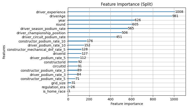
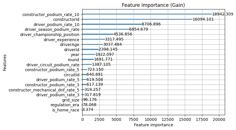
Tuning has reshuffled things quite significantly. The most striking change is that constructor_podium_rate_10 has jumped to the top of gain, displacing constructorId from the position it held throughout every previous iteration. The model has shifted from preferring to know who the constructor is to preferring to know how they've been performing recently, which is a meaningful change in what the model considers most decisive.
The split counts have collapsed again compared to the pre-tuning model, with the tuned model making far fewer splits overall but extracting more information from each one. regulation_era and is_home_race sit at the very bottom of both charts with negligible counts, confirming they can go.
So where does that leave us overall? We started with a baseline AUC of 0.79 and a Brier score of 0.12. Through iterative feature engineering and hyperparameter tuning we've pushed that to 0.8886 and 0.0843 respectively. The features that actually moved the needle were constructor identity and rolling performance rates, driver form within the current season, and championship position as a composite signal. A lot of the features we tried along the way didn't add much on top of what the model already knew, which is a perfectly normal outcome and an important part of the story.
Not everything earns its place, and knowing what to drop is just as valuable as knowing what to add.
Testing time
We held out the 2025 set, now it's time to check how it's performed.
One important detail here: we can't just slice out the 2025 rows and apply the feature engineering in isolation. The rolling features for the first race of 2025 need the 2024 history behind them, so we run the full pipeline on the complete dataset first and then slice out 2025 afterwards. Get that order wrong and the model is predicting the Australian Grand Prix with no prior form data to draw on.
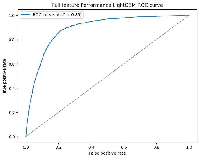
How did we do?
| AUC/ROC | Brier Score |
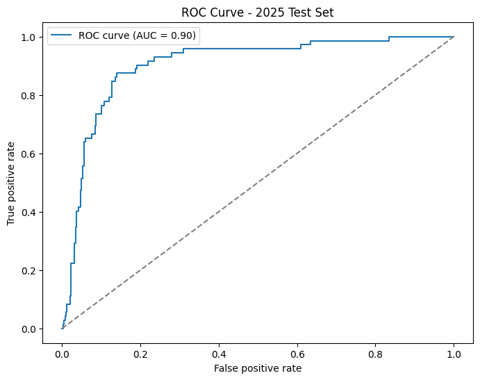
| 0.9048 (baseline: 0.79) | 0.0818 (baseline: 0.12) |
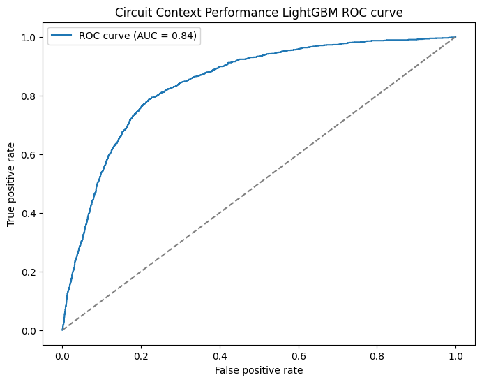
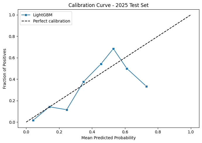
Against the held-out 2025 season the model performed really well. A 0.90 AUC on a completely unseen year tells us the model is confidently separating likely podium finishers from the rest of the field, and the ROC curve shape backs that up with a steep early climb before flattening out. The headline numbers of 0.9048 AUC and 0.0818 Brier actually come in slightly better than the walk-forward validation figures, which is the best case outcome. The model generalised cleanly to a new season rather than overfitting to patterns in the training years.
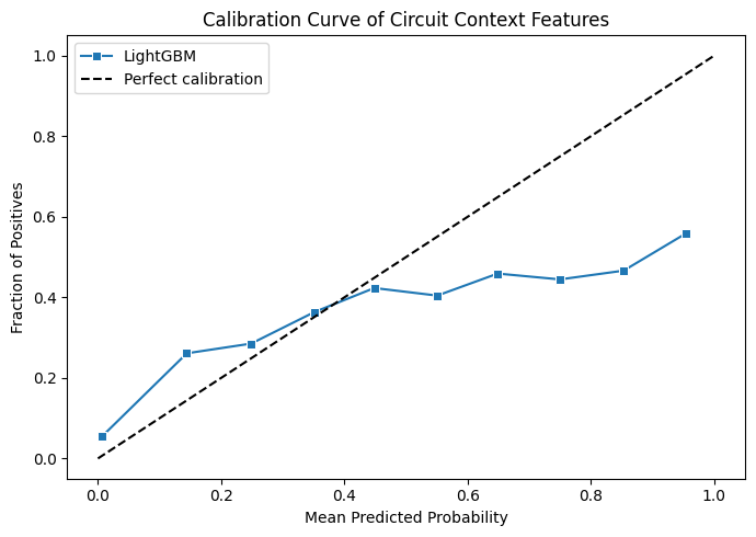
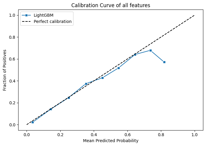
The calibration curve is noisier and more jagged than what we saw during cross-validation, but that's expected rather than concerning. During walk-forward validation we were pooling predictions across many seasons, giving each calibration bin thousands of samples to average over. For 2025 we have one season, roughly 24 races and around 400 rows. So each bin contains only a handful of predictions, therefore a few unexpected results in any bin is enough to swing the fraction of positives significantly.
Overall, it's a win!
Return to MLFlow
Remember how we setup MLFlow at the start? We haven't talked about it in a while so I'm sure you're wondering, why did we have to do that?
We actually set this up for a couple of different reasons. Remember at the start we had a quote from Adam Savage? Well, we didn't actually need to write anything down because this whole time we've been wrapping all of the training within the context of an MLFlow run.
This means that we have:
- The parent metrics of the average AUC/ROC
- Each child runs metrics
- The details of all of the training data used for each run
- Each run is tagged with the improvements that were made and what data was used
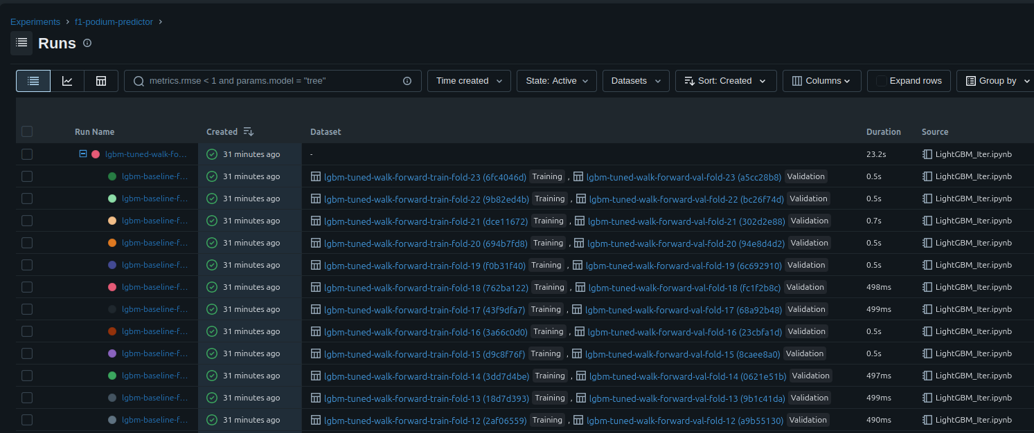
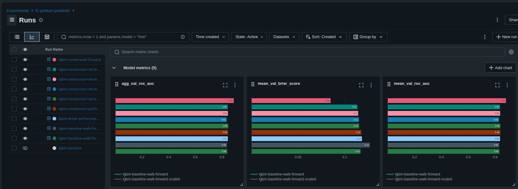
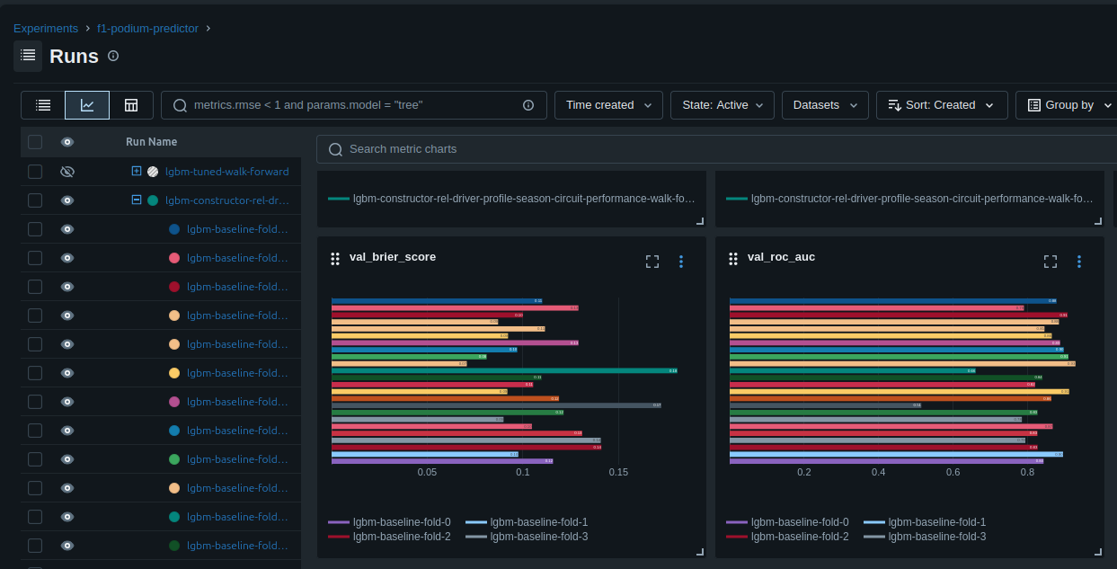
This is really useful, because we know not only how the model performs, but we have long term tracking outside of the notebook of why it performs. Which honestly is just as if not more useful.
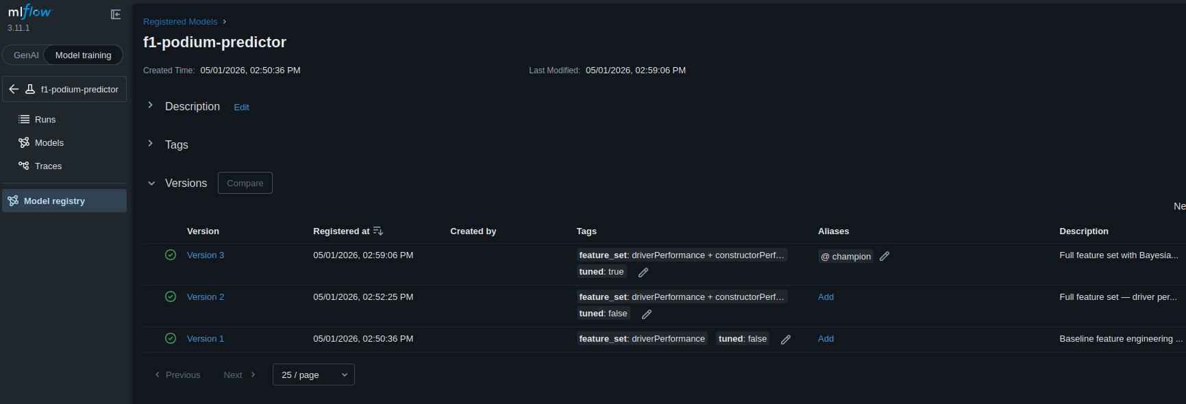
The last major feature of MLFlow that is a big help to us is the model registry. What we do is we've chosen particular runs of the model and promoted those to put them in the model registry and versioned them. We added a little bit of code as well to this registration step that generates the ONNX that we'll use to serve the model later.
def RegisterModel(run_name, model_name, alias=None, description=None, tags=None):
    import onnxmltools
    from onnxmltools.convert.common.data_types import FloatTensorType

    client = mlflow.MlflowClient()
    run_id = mlflow.search_runs(
        filter_string=f"tags.mlflow.runName = '{run_name}'"
    )["run_id"].iloc[0]

    result = mlflow.register_model(
        model_uri=f"runs:/{run_id}/{run_name}",
        name=model_name
    )

    if alias:
        client.set_registered_model_alias(model_name, alias, result.version)

        lgbm_model = mlflow.lightgbm.load_model(f"runs:/{run_id}/{run_name}")
        initial_types = [("input", FloatTensorType([None, len(lgbm_model.booster_.feature_name())]))]
        onnx_model = onnxmltools.convert_lightgbm(lgbm_model, initial_types=initial_types, target_opset=12)

        with mlflow.start_run(run_id=run_id):
            mlflow.onnx.log_model(onnx_model, name=f"{run_name}-onnx")

    if description:
        client.update_model_version(
            name=model_name,
            version=result.version,
            description=description
        )

    if tags:
        for key, value in tags.items():
            client.set_model_version_tag(model_name, str(result.version), key, value)

    return result
This means that we have built models ready to go, and as soon as we want to change the deployed version, if built correctly, then all we need to do is push a new promoted version and move the alias
Next time...
We've done a lot this time, thankfully a lot of the detailed work is over now. It's largely infrastructure and architecture from here on out. Next time we'll go over ONNX, the details of hosting and how to track for drift.